

— Blogs —
—Products—
 Consumer hotline +8618073152920
WhatsApp:+8615367865107
Address:Room 102, District D, Houhu Industrial Park, Yuelu District, Changsha City, Hunan Province, China
Product knowledge
Time:2026-11-10 08:30:00 Popularity:1
An environmental monitoring network is a set of nodes sharing one clock, one address plan and one gap policy. Node density should be set by the distance over which a reading stops representing a decision, not by dividing an area by a round number. Most network failures are timestamp or coverage failures, not sensor failures.
A common sizing shortcut squares an area-to-spacing ratio. For 100,000 km² at 25 km spacing it quotes (100,000 / 25)² = 1600 stations, 2500 at 20 km and 10,000 at 10 km. The printed result cannot be reproduced from the printed expression — (100,000 / 25)² is 16,000,000, not 1600 — and the expression is not dimensionally consistent either: 100,000 km² divided by 25 km is a length of 4,000 km, and squaring a length does not produce a node count. Treat 1600 as a published shortcut, not a defensible calculation.

Figure 1. Outdoor Industrial LoRaWAN Gateway 16 Channels power supply via POE.
A grid of square cells with side s covers s² of area per node. At 25 km spacing each node covers 625 km², so 100,000 / 625 = 160 nodes, not 1600. The shortcut treated an area-to-length ratio as a dimensionless count and squared it; because the same 10× difference repeats at every spacing, comparing two rows reveals no arithmetic slip.
Illustrative calculation based on assumed site values, not a measured field record. Real networks are not square grids: terrain, access, power and the decision being supported all change the layout. Use the arithmetic to check an order of magnitude, not to order hardware.
An environmental monitoring network sized at 160 rather than 1600 nodes differs by an order of magnitude in capital cost, backhaul contracts and calibration labour; enclosures and site visits scale with node count, while the platform licence does not.
Spacing is a correlation question. If the quantity varies over 1 km — a local plume, a shaded hillside, an irrigation block — 25 km spacing cannot resolve it at any budget. If it is regional background changing over tens of kilometres, 10 km spacing spends power, SIM cards and backhaul on readings that add almost no information. Fix the decision distance first: how far apart can points A and B be before the difference stops changing a decision?
Use a paired pilot: co-locate two nodes for 7 days, then move them 1 km, 5 km and 25 km apart for 7 days each, recording the median absolute difference between their 10-minute means. Where that difference stops growing, the local signal has given way to the regional one. Check at least two wind regimes.
Without that measurement an environmental monitoring network has no defensible spacing; a round number from a catalogue is a purchasing convenience. Record the pilot distances and differences in the commissioning file as a baseline for later density changes.
Node count and gateway count are different numbers. One cabinet in this product class accepts 16 wired sensor inputs and holds 128 GB locally, with transmission that resumes at the break point and thresholds that can be set remotely. A separate DTU/RTU unit offers RS232, RS485 and SDI-12 ports alongside analog and switch I/O, so one project can mix serial and analog channels. Count the physical inputs, not the protocol names, when the channel list is written.
Take ten sites, each with one gas channel and one meteorological channel. Twenty channels exceed the 16 inputs of one cabinet, so the design needs a second aggregation point or a local logger at each site unless channels are dropped. Settle that in the interface list before ordering, not during commissioning.
A 4G router in the same family carries RS232 and RS485 traffic over Modbus TCP/RTU or MQTT. Confirm which configuration was ordered before assuming that "RS485" implies a particular uplink. Confirm every numeric value against the current datasheet for your unit.
A 4G edge gateway and a LoRaWAN gateway are different devices with different capacity limits. The 4G units described here gather wired serial channels and backhaul them over cellular; they do not receive LoRaWAN radio frames. A LoRaWAN gateway is sized by its channel count, spreading factor, packet interval and the duty-cycle or fair-use policy in force, so its node capacity cannot be derived from the RS485 polling budget below. If a design uses both, write two separate capacity calculations and confirm which gateway model was ordered before assigning nodes to it.
What travels from a node is a record, not a reading: device ID, channel ID, raw value, scale factor, unit, quality flag and timestamp source. A gateway forwarding only scaled values loses the raw word needed to re-decode a frame after a firmware revision — a data-model failure, not a communications failure. Store raw and scaled values together and version the register map, so an environmental monitoring network survives a firmware change.
Every channel on a shared serial bus consumes polling time. Assume 20 channels, a 9600 baud link, a request of 8 bytes, a response of 25 bytes, 3.5 character times of silence between frames, and 80 ms of device turnaround per transaction. One transaction occupies roughly (8 + 25) × 10 bits / 9600 ≈ 34 ms of line time plus 80 ms of turnaround, or about 114 ms. Twenty channels need about 2.3 s per full sweep, before retries.

Figure 2. 4G IoT Router Support RS485 RS232 serial port for smart industry, transportation, agriculture, weather.
A 60 s refresh looks safe at 20 channels and at 256, which is the trap: retry behaviour, not sweep time, is the constraint. At 10% retries a 256-channel sweep takes 32.1 s. Adding 200 ms of turnaround per transaction takes it to about 80 s, and a 20% retry rate on top to about 97 s; both exceed the interval, so the collector returns the previous value with a fresh timestamp. A stale value stamped as current is worse than a gap, because no quality flag fires.
Measure the sweep on the installed bus, not the bench: log elapsed time and retry count per poll and test the longest cable run with every channel active. Where the schedule cannot close, split the bus, shorten the channel list or lengthen the interval. Do not shorten the timestamp; in an environmental monitoring network an overrun is invisible in the exported series unless sweep time was recorded.
A network with ten nodes scheduled to report every minute has 14,400 node-intervals per day. If one node loses its uplink for 6 hours and two more are out for calibration during a 2-hour window, the loss is 360 + 2 × 120 = 600 node-intervals. Daily coverage is (14,400 − 600) / 14,400 = 95.8%.
Comparisons need two nodes valid in the same interval. If a 30-day comparison needs 43,200 paired intervals and only 34,560 have valid readings at both nodes, paired coverage is 80%. Uptime is a device metric; paired coverage is a dataset metric, and an environmental monitoring network is judged on its dataset, not on the number of powered enclosures.
Compute paired coverage per comparison, not once for the whole system. Two stations each at 98% uptime share about 96% of intervals when their outages do not overlap (0.98 × 0.98), and about 98% when they coincide exactly. State the denominator with every difference; only a missing reading reduces coverage, not a flagged one. A 3-minute clock offset can move 3 of every 10 one-minute samples into the adjacent 10-minute window, so an apparently valid pair can still be misaligned.
Clock source decides whether paired intervals exist at all. Two nodes whose clocks differ by 3 minutes can appear to agree on a slowly changing value and disagree completely during a fast plume that rises and falls inside those 3 minutes. Store the timestamp source with each record, and never present an interpolated value as a measurement.
Recovery policy decides what the gap means. Backfilling raw values preserves the record but hides the outage unless flagged; marking the gap leaves derived averages short unless the denominator is adjusted; interpolating produces a smooth series that must not be compared against a limit. Test which one the platform implements by pulling a known outage interval and comparing the raw store with the export.
Check the raw store against the export after any firmware change, since a silent scaling revision produces a plausible step across every node. An environmental monitoring network that never labels its gaps cannot distinguish an outage from a flat process, and will report a clean record during exactly the period a client asks about.
More nodes can reduce data quality. Each device needs its own address, and continuity on the data pair says nothing about supply voltage at the far end. Measure supply at the farthest sensor with the bus active, include cable loss and gateway draw, and keep a margin for cold-start current. An eleventh node fitted without that check can brown out the whole segment, making ten existing channels fail together.
Polling is the second limit, comparability the third: a node with a different inlet exposure, calibration convention or averaging interval cannot be compared with the others. An environmental monitoring network with 20 nodes and no shared acceptance method holds less usable data than one with 8 nodes and a documented register map.
Do not assume extra baud rates, an unlimited device count or a cable distance that was never measured. Provide the point count and locations, the receiver model, the cable route, the supply arrangement, the required refresh and the remote destination rather than inferring compatibility from the words RS485 and PLC. Verify the ordered configuration against the register map before the eleventh node is energised.

Figure 3. 8-in-1 Compact Ultrasonic Weather Sensor — PM2.5 PM10 Noise Environmental Monitoring Sensor.
Q1. How many stations does a 100,000 km² region need at 25 km spacing?
About 160 by an area-per-node calculation: each 25 km cell covers 625 km², so 100,000 / 625 = 160. A published shortcut quotes 1600 for the same case, but its expression does not reduce to a node count, and the difference is 10×. These are illustrative grid figures, not a layout; terrain, power and the decision distance change the answer.
Q2. Is one gateway enough for ten sites?
It depends on channel count, not site count. One cabinet accepts 16 wired inputs; ten sites with two channels each need 20 inputs unless a local logger aggregates them or channels are dropped. A separate DTU/RTU adds serial, analog and switch inputs for mixed channel types.
Q3. Why is paired coverage lower than device uptime?
Comparisons need two nodes valid in the same interval. In a 30-day example, 34,560 of 43,200 paired intervals were valid, or 80%, even though individual node uptime was higher. Clock offsets, calibration windows and uplinks all reduce the paired denominator. Quote the paired figure with any network comparison.
Q4. Can I add an eleventh node to an existing bus?
Not without checking supply and polling. Each device needs a unique address, and continuity on the data pair does not prove adequate voltage. Measure supply at the farthest sensor with the bus active, include cable loss and gateway draw, and confirm the sweep still closes within the refresh interval.
Q5. Should gap values be interpolated?
No. Fix the recovery policy in advance: backfill raw values with a flag, mark the gap explicitly and adjust the averaging denominator, or exclude the interval. Local storage and transmission that resumes at the break point keep records through an outage, but timestamp quality and gap labelling decide whether the record is defensible.
Q6. What belongs in every network record?
Device ID, channel ID, raw value, scale factor, unit, quality flag and timestamp source. A gateway that forwards only scaled engineering values loses the raw value needed to re-decode a frame after a firmware revision. Version the register map whenever a channel is added, and keep the raw value with the scaled one.
A network is a shared record, not a map of dots. An environmental monitoring network stands or falls on things that do not appear on a site map: the address plan, the register map, one clock source, a poll sweep that finishes on time, and a gap policy written before the first outage. The 160 versus 1600 arithmetic moves a budget by an order of magnitude, and a polling schedule can pass on paper while delivering stale values with fresh timestamps. Size nodes by decision distance, measure the sweep on the installed bus, and report paired coverage with every comparison.
What the node count cannot tell you
An environmental monitoring network is specified by paired coverage and polling budget, not by area divided by a round number. The 1600 versus 160 node arithmetic moves a budget by an order of magnitude, two stations each at 98% uptime share about 96% of intervals when their outages do not overlap, and a 4G edge gateway is not a LoRaWAN gateway — each needs its own capacity calculation. A polling schedule can pass on paper while delivering stale values with fresh timestamps. Start with a paired pilot, fix the time source and register map, then set node density from the share of intervals that carry usable, contemporaneous values.
Sizing an environmental monitoring network? Send the site count, polling interval and uplink constraints through our contact page, and we will help you check the polling budget and paired coverage before you order gateways.
Prev:Wastewater Monitoring: Why Online and Lab Results Differ
Next:no more
Related recommendations
Sensors & Weather Stations Catalog
 Agriculture Sensors and Weather Stations Catalog-NiuBoL.pdf
Weather Stations Catalog-NiuBoL.pdf
Agriculture Sensors Catalog-NiuBoL.pdf
Water Quality Sensor Catalog-NiuBoL.pdf
Related products
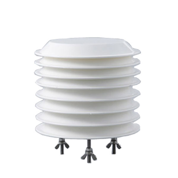 Combined air temperature and relative humidity sensor
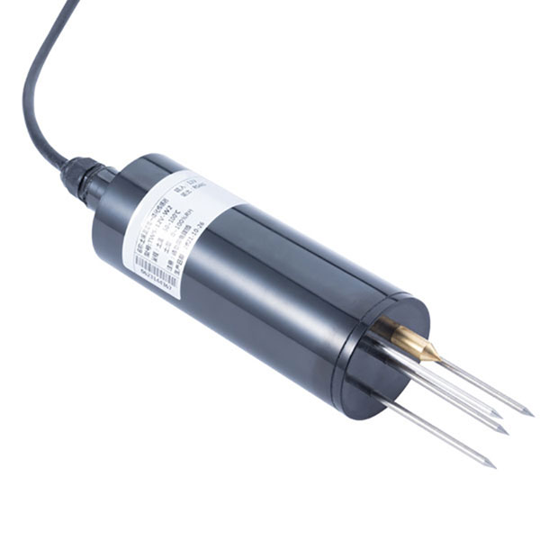 TDR Soil Moisture & Temperature Sensor for irrigation| RS485 |4-20mA| NBL-S-THR
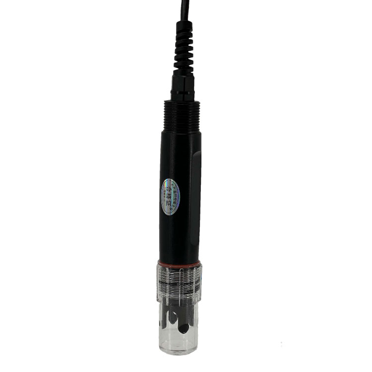 Soil pH sensor RS485 soil Testing instrument soil ph meter for agriculture |NBL-S-PH
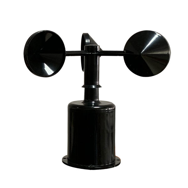 Wind Speed sensor Output Modbus/RS485/Analog/0-5V/4-20mA
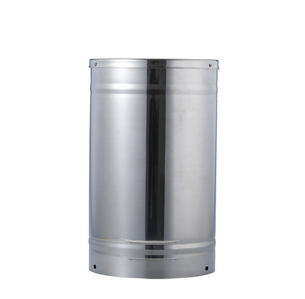 Tipping bucket rain gauge for weather monitoring auto rainfall sensor RS485/Outdoor/stainless steel
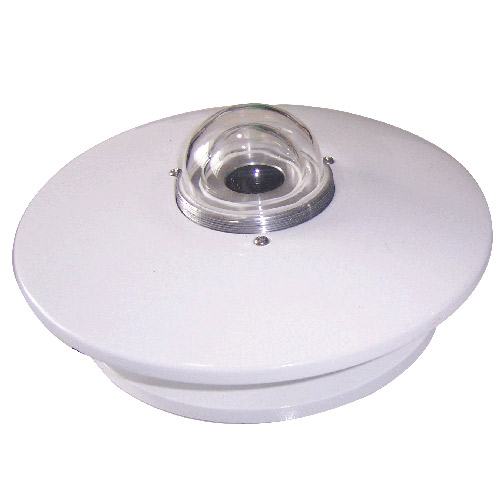 Pyranometer Solar Radiation Sensor 4-20mA/RS485


Screenshot, WhatsApp to identify the QR code
WhatsApp number:+8615367865107
(Click on WhatsApp to copy and add friends)